---
title: "Camera spectral response"
subtitle: "Full-spectrum Olympus E-M1"
author: "Pedro J. Aphalo"
date: 2024-12-20
date-modified: 2024-12-20
toc: true
categories: [equipment, cameras]
keywords: [LED light, ultraviolet, visible, infrared]
format:
html:
code-fold: true
code-tools: true
lightbox: auto
image: images/RawDigger-window.jpg
license: "CC BY-SA"
editor:
markdown:
wrap: 72
abstract: |
This page contains notes about my assessment of the spectral response of a full-spectrum-converted Olympus E-M1 mirrorless camera. The approach I used is based on LEDs emitting ultraviolet-A radiation, visible light and near infrared radiation of different wavelengths. A white target illuminated with the different LEDs was photographed. The relative signal values for red, green and blue sensor channel extracted from raw images obtained under illumination with different LEDs are presented as a normalised tri-chromatic response spectrum. _This page is subject to revision and will change in coming weeks_.
freeze: auto
draft: false
---
::: callout-note
::: {style="float: left; padding-top: 10px; padding-right: 10px;"}
{width="75" fig-alt="Strong-optical-radiation ISO warning sign."}
:::
This page is still a draft, not only of the text. Data are incomplete and may contain
errors even if I have been careful. As any work in progress the contents of this
page may drastically change, even in some of the conclusions. The methods are
described in detail, and, I hope already fully reproducible.
:::
{{< include /_includes/uva-warning.qmd >}}
{{< include /_includes/folded-code-tip.qmd >}}
## Introduction
I have been using a full-spectrum modified Olympus E-M1 camera since 2016. The
modification to increase the range of wavelength sensitivity was based on
replacement of the built-in "UV IR cut" filter with UV and NIR transparent
glass. The RGB filters of the Bayer array remained on the sensor. This results
in a colour cast in the VIS region and false colour in the UVA and NIR regions.
The colour cast in normal visible photography can controlled by means of an
external filter úsed to substitute for the removed internal one. In the tests
described here, no such filter was used, and the extended range of walengeths to
which the camera responds after modification was available.
Interpreting the false colours in UV and "far-red" is rather difficult as they
tend to vary vary to some extent between camera models. The interpretation would
be easier with knowledge of the spectral response of the RGB channels of the
modified camera. A low cost approach is to use LEDs emitting at different
wavelengths instead of a very expensive spectrograph (see page [Camera
objectives for digital UV photography](../lenses/lenses-for-uv.qmd)). Of course
the approach has limitations as the emission peaks of LEDs are rather broad and
the nominal wavelength of emission can differ from the actual one. The "loose"
LED wavelength specifications are common in generic LEDs from small suppliers,
but these suppliers do carry what seem to be "off-type" LEDs or from unusual
wavelength bins. The actual wavelength needs to be measured, but otherwise these
"generic" LEDs provide a way of obtaining LEDs emitting at wavelengths in
between the typical ones.
A recently announced commercial spectral imaging system is based on the use of
nine types of LEDs (eight colours and white) switched-on sequentially instead of
an spectral camera ([Rayn vision system
camera](https://rayngrowingsystems.com/products/rayn-vision-camera/) from [Rayn
Growing Systems](https://rayngrowingsystems.com/)). It is based on a 1/4"
1‑Megapixel (1280 x 800) sensor (OV9281, Omnivision, Santa Clara, CA, USA), as
used in some cameras for the Raspberry Pi available for around 25--35 u\$s ready
to plug-in with lens included. The camera sensor choice would be reasonable for
a cheap system as it has a global shutter. However, other sensors from
OmniVision could offer higher definition (5 Mpix or 9 Mpix), better dynamic
range and better low-light and infrared sensitivity. The example images from the
Rayn system are of individual small plants, the ability to image multiple plants
or single large plants with high enough resolution can be extremely useful for
phenotype screening and condition assessment, respectively.
The Rayn vision system uses eight wavelengths ranging from 475 nm to 940 nm at
the LEDs' peak of emission. This system seems overly expensive at a list price
of over 8000 u\$s. It is delivered with open-source software. On the other hand,
the approach seems easy to implement at a relatively low cost. In fact, nothing
prevents the use of a camera with a sensor with higher resolution and better
light sensitivity. The range of the Rayn system LEDs does not cover the
UVA-violet-region and the blue region only in part, but extends into the NIR.
Using a full-spectrum converted or other suitable camera it would be possible to
extend the wavelength range further than that provided by any single
hyper-spectral camera that are commercially available. With suitable filters on
the camera lens to block the light used for excitation and powerful enough
LED-based light sources one could image fluorescence excited by different
wavelengths, i.e., obtain spectral data using fluorescence as a reporter instead
of reflection. This approach has been used *in vitro* to characterise plant
photoreceptors. More relevant to whole plants, chlorophyll fluorescence informs
about photosynthesis activity and state and has also been used as a reporter of
UV transmittance of leaves' epidermis.
Thus I aimed at preliminarily testing the suitability of camera, lens and LEDs.
The specific aims of the test were: 1) to test the range of response of the
camera with a lens I normally use, 2) measure the
*relative* sensitivity of the red. green and blue sensor channels to
radiation of different wavelengths, and 3) assess if spectral imaging would be
feasible using LED illumination as sources of "monochromatic" light.
## Methods
### R code
The code below attaches R packages to be used and reads in the measured
response data and the metadata describing the LEDs and filters used.
```{r, message=FALSE}
library(dplyr)
library(tidyr)

library(photobiology)
library(photobiologyWavebands)
library(photobiologyFilters)
library(photobiologyLEDs)
library(ggspectra)
photon_as_default()

library(ggplot2)

knitr::opts_chunk$set(
  fig.width = 7, fig.height = 4, dev = "svg", out.width = "95%", message = FALSE
)
theme_set(theme_bw() + theme(legend.position = "top"))
```
```{r}
# read files saved using RawDigger: RGB values, shutter speed, aperture and ISO
main_samples.df <- read.csv("sampled-regions.csv")
green_samples.df <- read.csv("green_samples.csv")
new_samples.df <- read.csv("new_samples.csv")
nir_samples.df <- read.csv("NIR_827_samples.csv")
new_samples.df$Id <- new_samples.df$Id - 1L
pixel_samples.df <- rbind(main_samples.df, green_samples.df, new_samples.df,nir_samples.df)
# colnames(pixel_samples.df)
```
```{r}
# each raw image file has a matching entry with information about LED and filter used
if (file.exists("frames-metadata.csv")) {
  frames_metadata.df <- read.csv("frames-metadata.csv") |>
    mutate(LED.Id = paste(LED.Id, Wavelength, sep = "."))
} else {
  # save template for manual editing
  filenames.df <- unique(pixel_samples.df["Filename"])
  write.csv(filenames.df, file = "frames-metadata.csv", row.names = FALSE)
}
# colnames(frames_metadata.df)
```
```{r}
# The description of each LED is in a separate file
if (file.exists("leds-metadata.csv")) {
  LEDs_metadata.df <- read.csv(file = "leds-metadata.csv")
} else {
  # save template for manual editing
  LEDs_metadata.df <-
    unique(frames_metadata.df[c("LED.Id", "LED", "Wavelength", "wl.real")])
  write.csv(LEDs_metadata.df, file = "leds-metadata.csv", row.names = FALSE)
}
```
```{r, message=FALSE}
# Join data with metadata
camera_response.df <- left_join(pixel_samples.df, frames_metadata.df)
# colnames(camera_response.df)
save(camera_response.df, file = "camera-response-df.rda")
```
### Camera and lens
A mirrorles digital camera (E-M1 (Mk I), Olympus, Japan) camera from
2013, converted to full-spectrum (by [DSLR Astro TEC](http://www.dslr-astrotec.de/index-eng.html)) was used. The camera has a
4/3" sensor with an effective resolution of 16 Mpix. For the tests a
Sigma 30 mm 1:2.8 DN A lens was used. This modern autofocus lens
transmits UV-A1 radiation rather well, much better than any other modern
lens for this system. For the test at 340 nm, a different lens with
deeper UV transmission was used: a Soligor 35 mm 1:3.5 from the 1960's
on M42 mount (s.n. 9700437) was attached to the camera with a helicoid
adpater and aperture and focus set manually.
The camera was mounted on a copy stand (MS-Repro, Novoflex, Memmingen,
Germany) through a macro focusing rail (MFR-150, Sunwayfoto, Zhongshan
city; China). On the camera an Arca-type base-plate specific to the
camera model (generic from AliExpress) ensured alignment.
::: {#fig-copy-stand}
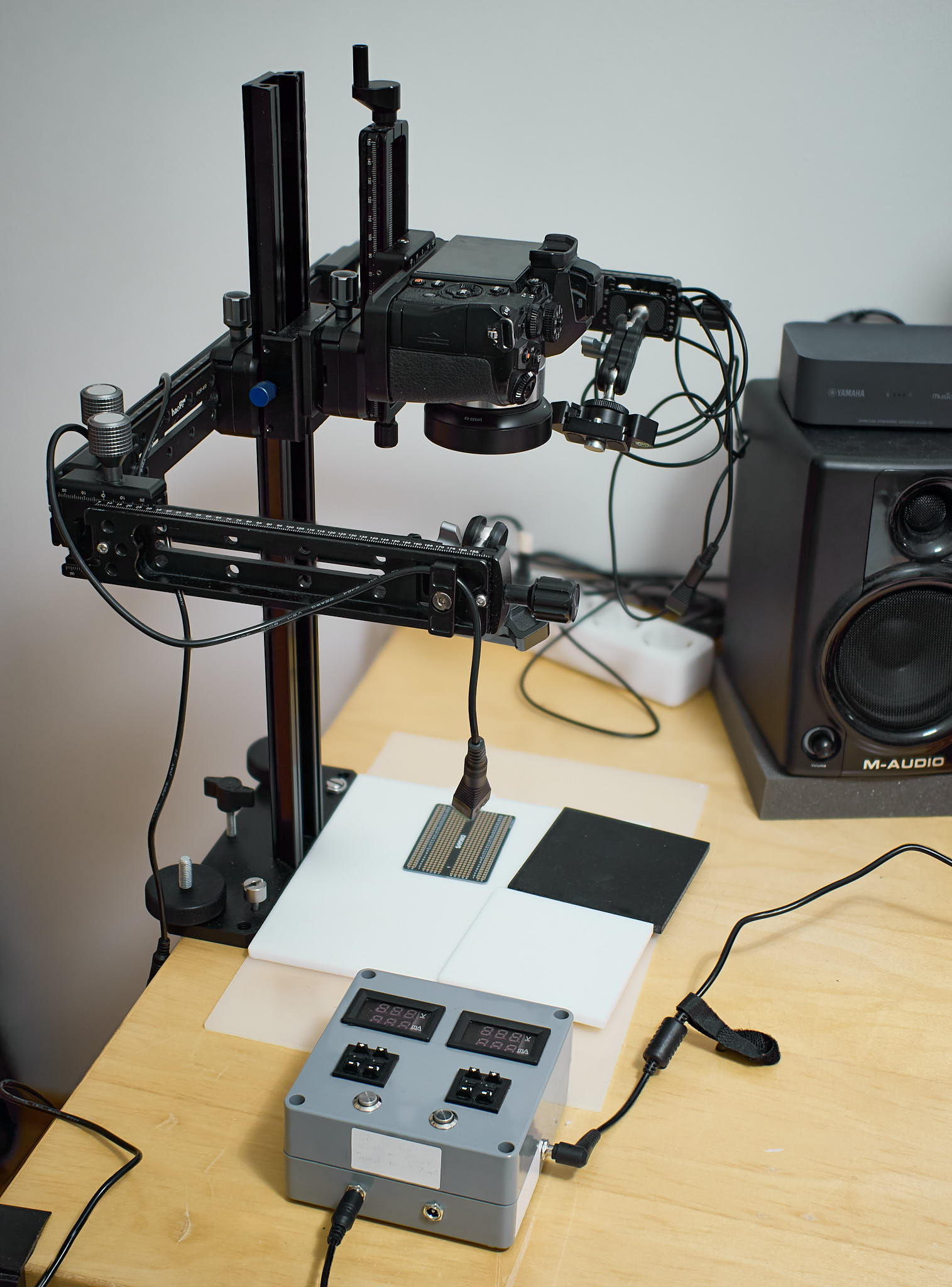{fig-alt="General view of the copy stand with a camera in place." width=67%}
Copy stand with the camera and rails for supporting two LEDs. The grey device near the front edge of the table is a custom-built LED driver.
:::
### LEDs
On the copy stand a solid support for the LEDs was assembled using Arca
type rails and clamps (Haoge HDR-400, FITTEST D290 angle clamps, XILETU
QR-50B two way clamps, generic NDR-200 nodal rails, all from
AliExpress), and small "magic arms" (UURig, AliExpress). The LEDs were
kept in place by magnets making swapping them fast and easy. LEDS in SMD
packages were used, soldered onto star-boards, and the star boards
mounted onto small aluminium heat-sinks (SA-LED-113E black anodized,
OHMITE, Rolling Meadows, Illinois, USA) using self-stick pre-cut thermal
transfer pads (LP0001/01-TG-R373F-0.25-2A-ND, T-Global Technology,
Lutterworth, U.K.). A small self stick magnetic attachment point (13 mm,
Magsy, Fryšták, Czech Republic) was fixed to the back of the heat sinks.
Small but strong magnets (13 mm NdFeB pot magnets, Magsy) were used on
the "magic arms".
::: {#fig-LED layout-ncol=2}
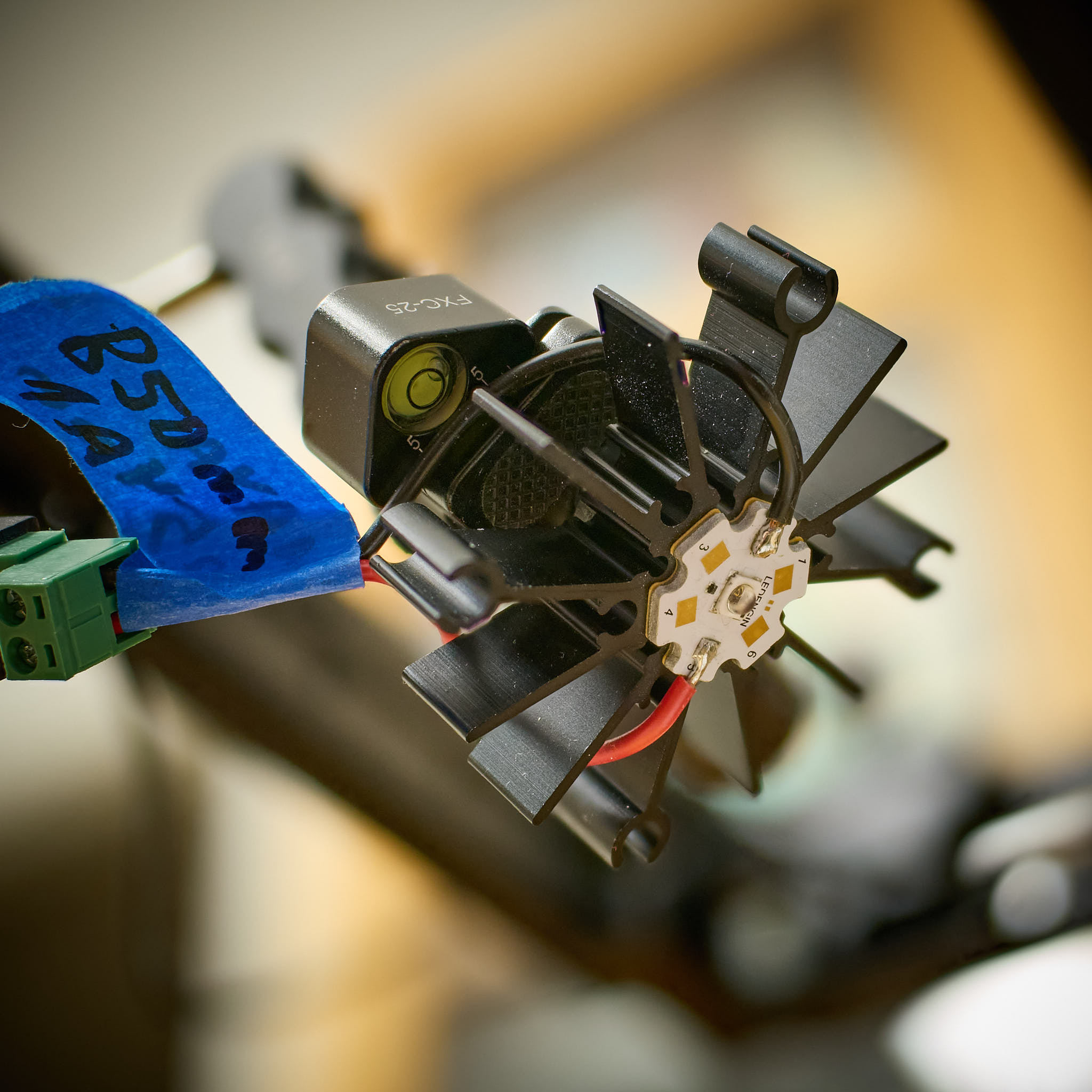
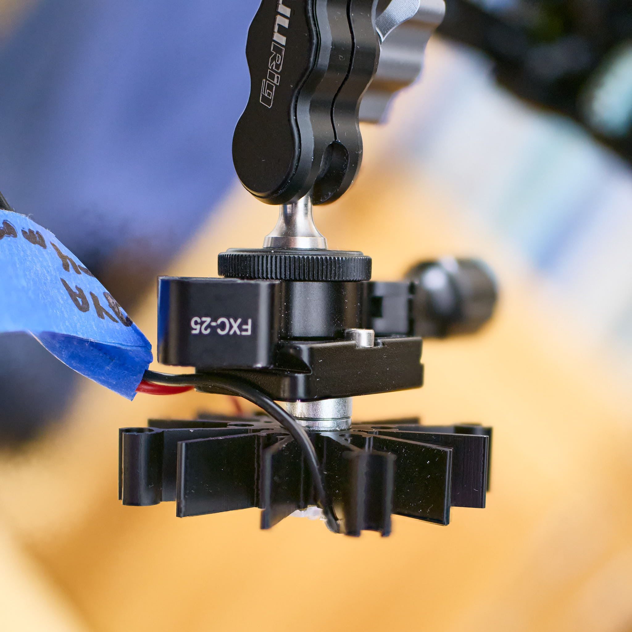
One LED in place ready to be used. It is held in place by a magnet. As the magnet and ferrous attachment point are of the same diameter, the positioning is easily repeatable.
:::
The `r nrow(LEDs_metadata.df)` LEDs used are described in @tbl-leds. The
emission spectrum of each LED used was measured with an array
spectrometer (Maya 2000Pro, Ocean Optics, USA) and are shown in the Appendix.
If you intend to use any UV-A or strong violet LEDs please read @wrn-uva
beforehand.
The measured wavelength, in some cases differed by more than 10 nm from the
nominal value, these differences were much smaller for LEDs obtained from big
distributors like Mouser, Digikey, Farnell, TME, etc., and large only for some
AliExpress sellers and LED types. Using nominal wavelengths results in a ragged
curve, while using actual wavelengths resulted in a very smooth curve.
```{r}
#| label: tbl-leds
#| tbl-cap: LEDs used. Those lacking a value in part "Code" column are generic parts lacking an official designation or known manufacturer part number. The use of generic LEDs does not affect the results as the peak of emission was measured for each LED using the same spectromter. In the designation of package "Type", SMD stands for surface mounted device and the four digits are the footprint such that, for example, 3535 means 3.5 mm $\times$ 3.5 mm. The maximum current $I_\mathrm{max}$ is the maximum recommended operating current by specification, assuming suitable cooling, expressed in milli amperes. Wavelengths are expressed in nanometres. Column "LED" gives the manufacturer of the LED chips when known. For generic LED types the values in the "LED" column must be taken with a grain of salt. **Notes** _a_ LEDs to be used when deliverred. _b_ This LED has a significantly higher power rating than single chip ones as it has 4 LED chips connected in series.
#|
knitr::kable(LEDs_metadata.df[order(LEDs_metadata.df[["Wavelength"]]) , c("Wavelength", "LED", "Type", "I.max", "Code", "Supplier", "Notes")],
             row.names = FALSE, align = "cll")
```
The LEDs were driven using a custom-built constant current controller
based of solid-state drivers (RCD-24-0.350, Recom Power, Gmunden,
Austria) and voltage and current monitored.
The targets, the camera and the LED positions remained unchanged durings
tests, carried out in a darkened room, keeping fluorescent objects at a
distance and for UV and NIR using band-pass and long-pass filters on the
camera lens, respectively.
### White, black and pattern targets
Two white-reference targets were used side by side ([@fig-BW-targets]). Each one a
slab of white PTFE 6 mm-thick with the surface sanded with 600 grit wet-dry sand
paper to obtain a matte surface. A 6 mm-thick black Nylon-slab painted with
"black deep mat" camera paint (Tetenal kameralack Spray 105202, seems no longer
available) was used as the black reference target. A
small printed circuit board, with a black-coloured mask and a clear plastic film
ruler were also added to facilitate focusing.
::: {#fig-BW-targets}
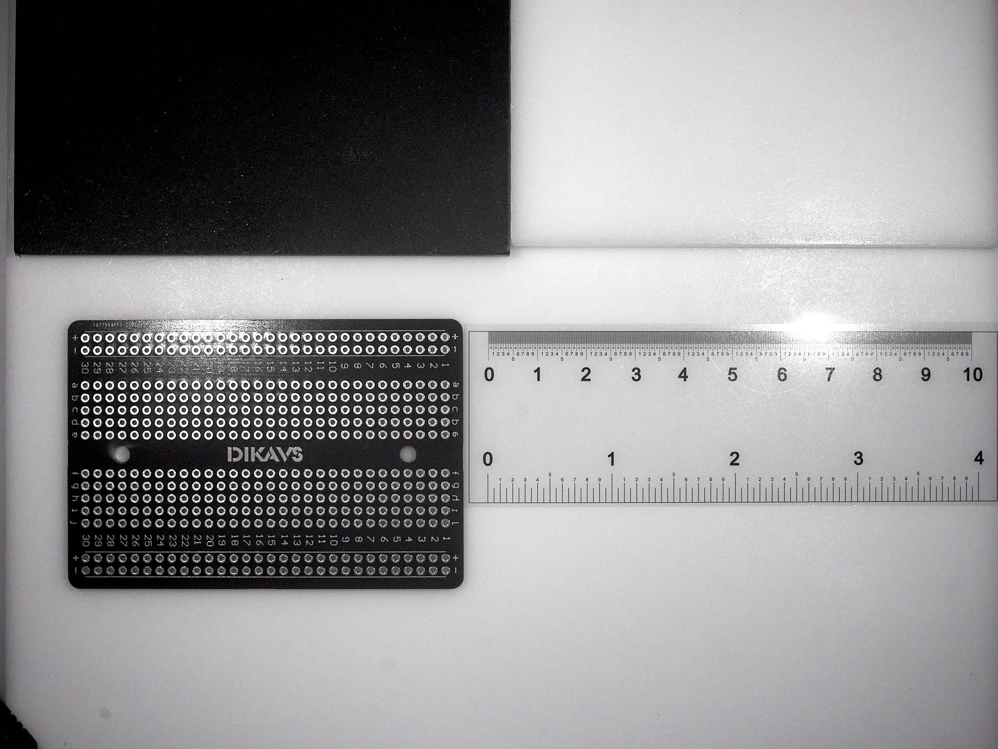{fig-alt="Black and white backgrounds, a small black PCB (unpopulated) and a clear ruler with black text and markings." width=67% fig-align="center"}
Targets used photographed in NIR shown after white balancing. Upper scale on the ruler shows centimetres and the lower one inches. The spacing of holes in the printed circuit board is 2.5 mm.
:::
### Image sampling
As the target and light sources, or camera were not moved, the sampling
was done at the same two locations in every image. Two well illuminated
areas, 500 x 500 pixels in size were sampled with [RawDigger](https://www.rawdigger.com/) (RawDigger Research Edition, version 1.4.9 for Windows, LibRaw LCC, ), and
the results of the sampling saved to two files, as the photographs were
acquired in two separate sessions.
::: {#fig-rawdigger}
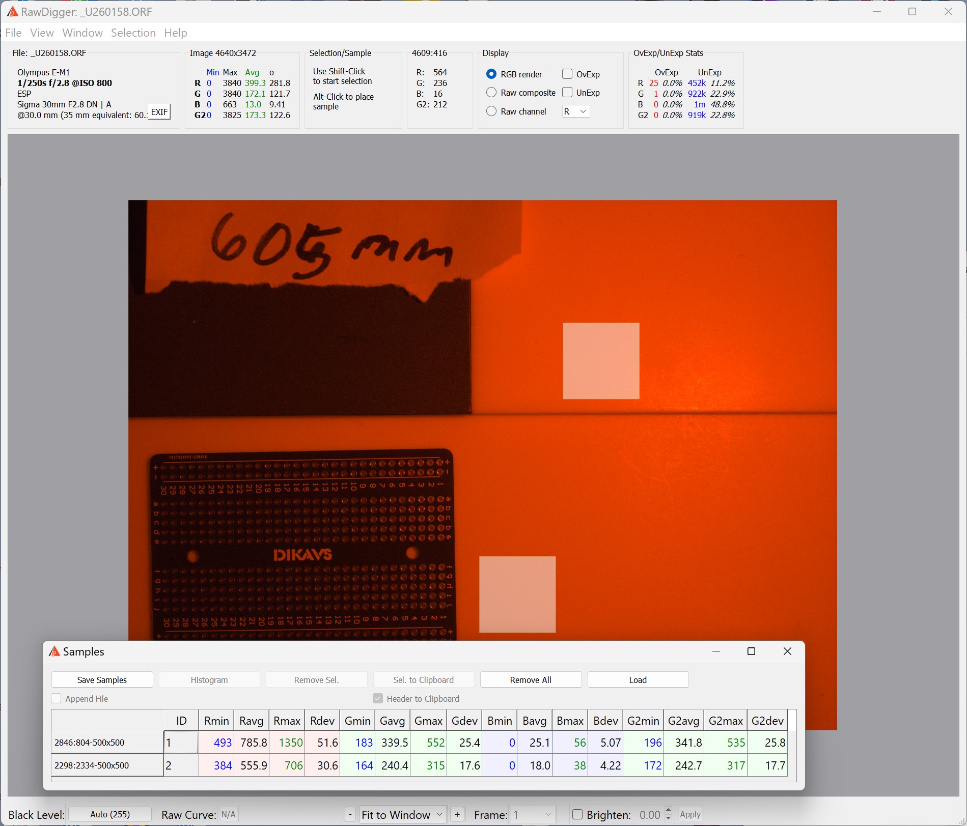{fig-alt="A view of the user-interface of the RawDigger program." width=67% fig-align="center"}
RawDigger with one photograph open. The two light-colored squares are the two sampled regions and the pop-up window shows the computed values for the two samples. From the pop-up the data were saved or appended to a .csv file.
:::
### Additional tests
All the test images were obtained using auto-focus and auto-exposure
settings with no manual exposure compesation. In some cases bracketing
was used, but the bracketed were not better exposed than the ones
exposed according to camera automation. Focusing worked in all cases,
except 340 nm, where the Sigma lens did not transmit enough to obtain a
well exposed image even at ISO 26500. At 940 nm, autofocus hunted to
some extent, but did work most of the time. The target included high
contrast features.
## Results
::: callout-note
# Normalise data
```{r}
camera_response.df |>
  mutate(RGB.sum = Ravg + Gavg + Bavg,
         Ravg.rel = Ravg / RGB.sum,
         Gavg.rel = Gavg / RGB.sum,
         Bavg.rel = Bavg / RGB.sum) |>
    select(Filename:Id, ISO:Aperture_Value, LED.Id:Bavg.rel) -> camera_response_rel.df
```
:::
The normalised data describe the relative sensitivity of the red (R),
green (G) and blue (B) channels of the camera sensor at different
wavelengths (@fig-rel-response). At each wavelength, the average pixel
values are expressed relative to the sum of the pixel values for R, G, B
channels. These values even if not describing the quantum efficiency of
the sensor, can help interpret the colours obserbed under nearl
monochromatic light. This is specially useful outside the visible range
of wavelengths that create a false-colour rendition on the photographs.
```{r, warning=FALSE}
#| label: fig-rel-response
#| fig-asp: 0.5
camera_response_rel.df |>
  select(-RGB.sum) |>
  filter(! Filename %in% c("_U250126.ORF", "_U250126.ORF", # sigma lens blocks 340 nm
                           "_U250091.ORF", "_U250088.ORF", # fluorescence in image
                           "_U250128.ORF") # underexposed
         & Id == 1) |>
  pivot_longer(cols = c("Ravg.rel", "Gavg.rel", "Bavg.rel")) |>
  ggplot(aes(Wavelength, value, colour = name)) +
  geom_line() +
  geom_point() +
#  facet_wrap(facets = vars(Id), ncol = 1) +
  wl_guide(ymin = -0.02, ymax = 0) +
  scale_color_discrete(direction = -1) +
  scale_x_wl_continuous(n.breaks = 6) +
  scale_y_continuous(name = "Raw pixel signal (relative to RGB sum)")
```
As response values are normalised, an alternative presentation approach
is to use stacked area plots (@fig-rel-response-stacked).
```{r, warning=FALSE}
#| label: fig-rel-response-stacked
#| fig-asp: 0.5
camera_response_rel.df |>
  select(-RGB.sum) |>
  filter(! Filename %in% c("_U250126.ORF", "_U250126.ORF", # sigma lense blocks 340 nm
                           "_U250091.ORF", "_U250088.ORF", # fluorescence in image
                           "_U250128.ORF") # underexposed
         & Id == 1) |>
  pivot_longer(cols = c("Ravg.rel", "Gavg.rel", "Bavg.rel")) |>
  ggplot(aes(Wavelength, value, fill = name)) +
  geom_area(alpha = 0.67) +
#  facet_wrap(facets = vars(Id), ncol = 1) +
  scale_fill_discrete(direction = -1) +
  scale_color_discrete(direction = -1) +
  scale_x_wl_continuous(n.breaks = 6) +
  scale_y_continuous(name = "Raw pixel signal (relative to RGB sum)",
                     sec.axis = dup_axis(name = character(),
                                         breaks = c(0, 1/3, 2/3, 1),
                                         labels = c("0/1", "1/3", "2/3", "1/1")))
```
## Discusion
### Approach
The approach of using LEDs works well as long as the wavelength value
used for calculations and expressing the observed RGB values is the exact one,
measured on the LEDs actually used,
rather than the nominal value reported in data sheets or informally in
sellers' descriptions (or measured on other LEDs of identical type and brand). The
peaks of emission of LEDs are rather broad, with half maximum full width
(HMFW) in the range 10 to 20 nm, limiting wavelength resolution of the
obtained camera spectral response characterization.
As the results from the two different sample areas were almost
identical, expressing the results as normalised relative sensitivities
makes the method rather insensitive to small changes in luminance and
setup geometry. The data are much easier to collect than actual quantum
efficiencies but are not useful to predict responses under light sources
that include a broad range of wavelengths.
For wavelengths at which camera sensor sensitivity is low or LED
emission weak room stray light can be a problem to be aware of. In
particular, under UV, visible fluorescence induced by absorbed UV
radiation needs to avoided.
One thing to be aware of is that the voltage drop across LEDs depends on
wavelength: as the energy per photon increases towards shorter
wavelengths the voltage drop increases. Some sellers correctly advertise
typical 3535 SMD LEDs as having a power rating of 1--3W. These LEDs are
rated at a maximum current of 700 mA consistently across wavelengths,
and consequently, IR LEDs are close to 1W power while blue, UVA and
white emitting LEDs are close to 3W power. In contrast, Ledengine/OSRAM
LEDs in the LZ1 series have a more even power rating across wavelengths
as the maximum allowed current increases with wavelength.
::: callout-tip
# LED suppliers
Buying LEDs from AliExpress sellers has the advantage of availability of
LEDs emitting at a broad range of wavelengths, including those
intermediate between the usual ones available through major distributors
in small quantities from stock. On the other hand, while LEDs bought
from distributors and reputable sellers are well described in technical
data sheets, the information provided by AliExpress sellers is usually
incomplete or even totally missing.
This means that wavelength tolerances can be broad and power ratings
suspect in the case of some AliExpress sellers. However, in my
experience in all cases LEDs from AliExpress sellers have been fully
functional.
:::
### Camera response
The response curves obtained are similar to what can be expected by
normalising those published for sensor detector arrays. By using a
converted camera and extending the test into the UV-A and NIR regions,
it is possible to see why the false colour for UV-A at 340 nm is yellow
and purple at 385 nm. We can also see why at wavelengths of 840 nm and
longer, images taken with this full-spectrum converted camera are
monochromatic.
### Next steps
The wavelength resolution in the range 950 to 1050 nm is less than at other
wavelengths but as response seems flat the wavelenth coverage is now good
enough. For quite a few LEDs I was using wavelengths from specifications, but I
have measured them with a spectroradiometer and I have updated the computations,
@fig-rel-response and @fig-rel-response-stacked with their true peak
wavelengths. I still need to update the LED figures and table in the Appendix
with the newly measured emission spectra and information on all LEDs used.
The method is fast and simple enough to be applied to other cameras,
full-spectrum converted and off-the-shelf, for comparison. Automation
would require electronic switching of LEDs in place of the current
manual swapping of LEDs. Attaching them with magnets as I am doing
helps a lot in speeding the process. The sensor response to exposure
seems to be linear when extraction the raw sensor "counts" with
RawDigger, so as long as there is no clipping, the normalised relative
sensitivity of the three channels does not change wihtin $\pm 2$ EV or
more (the data points from bracketed exposures are in the figures but
invisible because they overlap).
Ultimately, the aim is to develop an approach to spectral imaging based
on the use of light sources of different wavelengths and a normal camera
instead of a spectral camera. Thus, tests with plants, flowers and other
objects will be needed. These objects are more difficult than the PTFE
slabs and black-painted objects used for the tests reported here as they
can fluoresce.
As a caveat, assembling the "image cube" possibly requiring alignment
will be a further challenging step, possibly doable with
[plantCV](https://plantcv.org/) or other software. So, image analysis
will need to be also developed based on existing tools.
## Conclusions
1) The range of usable wavelengths into the UV region is mostly limited
by the lens I used, and in the NIR by the camera sensor.
2) In the UV the sensitivity of the blue channel rapidly decreases
with decreasing wavelength reaching nearly zero while that of red
and green channels become nearly the same ($\approx 0.5$), yielding
the typical yellow false colour at 340 nm. In the NIR, at the
opposite end of the spectrun at wavelengths of 840 nm and
longer all three channels had equal sensitivity ($\approx 0.33$),
as expected from the lack of false colour.
3) The camera and lens automation worked well across the whole
range of wavelengths tested, except that autofocus was sluggish
at 1005 nm.
_Thus, using LEDs for low-cost hyperspectral imaging should be possible, but
will require the development of a system for switching LEDs and triggering
the shutter: custom assembled LED arrays of 12 channels are relatively
easy to obtain and not too expensive but do not have the best geometry as
LED chips of each channel are in a row in the array._
On paper at least, the Ryan "hyperspectral" camera system seems to use an
unnecessarily weak camera sensor compared to the price and the sophistication of
other components. I may be wrong as the sensor has fast readout and a global
shutter, that taken together should allow acquiring the images very fast. It
uses eight colours and white light. For the test presented here I used LEDs with
peak of emission at `r length(unique(camera_response_rel.df$Wavelength))`
different wavelengths. In actual use for spectral imaging, in most cases a
smaller set of wavelengths would need to be selected to reduce the amount of
data as contrary to most true hyperspectral cameras, we also have high spatial
resolution.
It may appear counter-intuitive, but assessing colour is easier than assessing
overall reflectance as it does not depend on irradiance. As long as we have a
set of greyscale references usable across all wavelength or if we can assume a
linear sensor response to ligh, we can estimate reflectance. With whole plants,
with leaves displayed at multiple angles and facing multiple directions, the
irradiance at their surface is very difficult to keep uniform, even in a fully
diffuse light field because of mutual shading. In contrast, mutual shading
changes the light spectrum only minimally, if at all, when using a single-colour
light source. This is in contrast with the change in spectrum caused by mutual
shading of plants in sunlight and in white light. An important question is if a
diagnosis/image-analysis approach based only/mainly on colour would be effective
in detecting all the features of interest.
## Appendix
```{r}
#| label: tbl-frames
#| tbl-cap: LEDs, filters and conditions used for each image. Lens, SGM30 = Sigma 30 mm 2.8 DN A; SLG35 = Soligor 35 mm 3.5. Column LED.Id provides a cross-reference to @tbl-leds.
knitr::kable(frames_metadata.df[order(frames_metadata.df[["Wavelength"]]) , c("Filename", "Wavelength", "LED.Id", "Filter", "Lens")],
             row.names = FALSE, align = "cll")
```
```{r, warning=FALSE}
#| label: fig-filters
#| fig-cap: Spectral transmittance of the four filters used as indicated in table @tbl-frames.
filters.mspct[c("Heliopan_Red_25_SH_PMC_2.2mm_30.5mm",
                "Zomei_IR760_2.1mm_30.5mm",
                "Baader_U_filter_1.0mm_48mm",
                "Tangsinuo_Venus_2mm_30.5mm")] |>
  autoplot(facets = 2,
           annotations = list(c("-", "summaries", "boxes", "labels"),
                              c("+", "wls.labels", "peak.labels")))
```
```{r, warning=FALSE}
#| label: fig-leds-all
#| fig-asp: 0.5
#| fig-cap: Overview or the emission spectra of all LEDs used. See for details @fig-leds-uva, @fig-leds-blue, @fig-leds-green, @fig-leds-red and @fig-leds-nir.
leds.mspct[c("Roithner_DUV340_SD353EL",
             "LedEngin_LZ1_10UV00_365nm",
             "LedEngin_LZ1_10UB00_00U4_385nm",
             "LedEngin_LZ1_10UB00_00U8_405nm",
             "Epileds_3W_460nm",
             "Epileds_3W_470nm",
             "Epileds_3W_495nm",
             "LedEngin_LZ1_10DB00_460nm",
             "Epileds_3W_420nm",
             "Epileds_3W_430nm",
             "CREE_XPE_480nm",
             "Epileds_3W_520nm",
             "Weili_3W.nominal.525nm",
             "Weili_3W.nominal.550nm",
             "Weili_3W.nominal.555nm",
             "Epileds_3W_560nm",
             "Epileds_3W_590nm",
             "Epileds_3W_600nm",
             "Epileds_3W_620nm",
             "LedEngin_LZ4_40R208_660nm",
             "LedEngin_LZ1_10R302_740nm",
             "LedEngin_LZ1_10R602_850nm")] |>
  autoplot(idfactor = "LED",
           range = c(300, NA),
           annotations = "colour.guide") +
  theme(legend.position = "none")
```
```{r, warning=FALSE}
#| label: fig-leds-uva
#| fig-asp: 0.5
#| fig-cap: Emission spectra of the UVA and violet LEDs used as indicated in table @tbl-frames.
leds.mspct[c("Roithner_DUV340_SD353EL",
             "LedEngin_LZ1_10UV00_365nm",
             "LedEngin_LZ1_10UB00_00U4_385nm",
             "LedEngin_LZ1_10UB00_00U8_405nm")] |>
  autoplot(range = c(300, 450),
           idfactor = "LED",
           annotations = list(c("-", "summaries", "boxes", "labels"),
                              c("+", "peak.labels")))
```
```{r, warning=FALSE}
#| label: fig-leds-blue
#| fig-asp: 0.5
#| fig-cap: Emission spectra of the blue and cyan LEDs used as indicated in table @tbl-frames.
leds.mspct[c("Epileds_3W_460nm",
             "Epileds_3W_470nm",
             "Epileds_3W_495nm",
             "LedEngin_LZ1_10DB00_460nm",
             "Epileds_3W_420nm",
             "Epileds_3W_430nm")] |>
  autoplot(range = c(375, 575),
           idfactor = "LED",
           annotations = list(c("-", "summaries", "boxes", "labels"),
                              c("+", "peak.labels")))
```
```{r, warning=FALSE}
#| label: fig-leds-green
#| fig-asp: 0.5
#| fig-cap: Emission spectra of the green and yellow LEDs used as indicated in table @tbl-frames.
leds.mspct[c("CREE_XPE_480nm",
             "Epileds_3W_520nm",
             "Weili_3W.nominal.525nm",
             "Weili_3W.nominal.550nm",
             "Weili_3W.nominal.555nm",
             "Epileds_3W_560nm")] |>
  autoplot(range = c(450,650),
           idfactor = "LED",
           annotations = list(c("-", "summaries", "boxes", "labels"),
                              c("+", "peak.labels")))
```
```{r, warning=FALSE}
#| label: fig-leds-red
#| fig-asp: 0.5
#| fig-cap: Emission spectra of the orange and red LEDs used as indicated in table @tbl-frames.
leds.mspct[c("Epileds_3W_590nm",
             "Epileds_3W_600nm",
             "Epileds_3W_620nm",
             "LedEngin_LZ4_40R208_660nm")] |>
  autoplot(range = c(550,725),
           idfactor = "LED",
           annotations = list(c("-", "summaries", "boxes", "labels"),
                              c("+", "peak.labels")))
```
```{r, warning=FALSE}
#| label: fig-leds-nir
#| fig-asp: 0.5
#| fig-cap: Emission spectra of the near infrared LEDs used as indicated in table @tbl-frames.
leds.mspct[c("LedEngin_LZ1_10R302_740nm",
             "LedEngin_LZ1_10R602_850nm")] |>
  autoplot(range = c(650,NA),
           idfactor = "LED",
           annotations = list(c("-", "summaries", "boxes", "labels"),
                              c("+", "peak.labels")))
```


